Backpropagation- Example (part a)

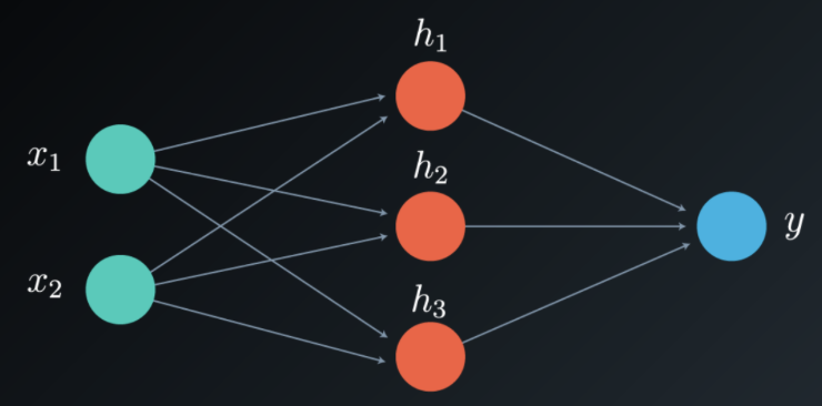
We will now continue with an example focusing on the backpropagation process, and consider a network having two inputs [x_1, x_2], three neurons in a single hidden layer [h_1, h_2, h_3] and a single output y.

The weight matrices to update are W^1 from the input to the hidden layer, and W^2 from the hidden layer to the output. Notice that in our case W^2 is a vector, not a matrix, as we only have one output.

The chain of thought in the weight updating process is as follows:

To update the weights, we need the network error. To find the network error, we need the network output, and to find the network output we need the value of the hidden layer, vector \bar {h}.

\bar{h}=[h_1, h_2, h_3]

Equation 8

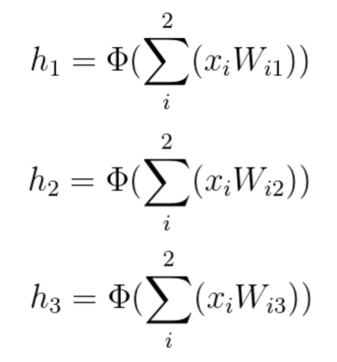
Each element of vector \bar {h} is calculated by a simple linear combination of the input vector with its corresponding weight matrix W^1, followed by an activation function.

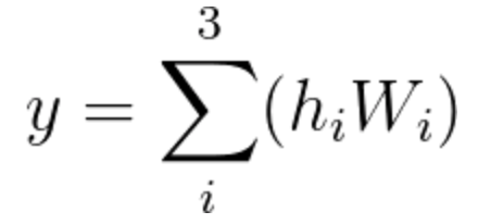
We now need to find the network's output, y. y is calculated in a similar way by using a linear combination of the vector \bar{h} with its corresponding elements of the weight vector W^2.

After computing the output, we can finally find the network error.

As a reminder, the two Error functions most commonly used are the Mean Squared Error (MSE) (usually used in regression problems) and the cross entropy (often used in classification problems).

In this example, we use a variation of the MSE:

E=\frac{(d-y)^2}{2} ,

where d is the desired output and y is the calculated one. Notice that y and d are not vectors in this case, as we have a single output.

The error is their squared difference, E=(d-y)^2, and is also called the network's Loss Function. We are dividing the error term by 2 to simplify notation, as will become clear soon.

The aim of the backpropagation process is to minimize the error, which in our case is the Loss Function. To do that we need to calculate its partial derivative with respect to all of the weights.

Since we just found the output y, we can now minimize the error by finding the updated values \Delta W_{ij}^k.
The superscript k indicates that we need to update each and every layer k.

As we noted before, the weight update value \Delta W_{ij}^k is calculated with the use of the gradient the following way:

\Delta W_{ij}^k=\alpha (-\frac{\partial E}{\partial W})

Therefore:

\Delta W_{ij}^k=\alpha (-\frac{\partial E}{\partial W})=-\frac{\alpha}{2} \frac{\partial (d-y)^2}{\partial W_{ij}}=-2 \frac{\alpha}{2}(d-y) \large \frac{\partial (d-y)}{\partial W_{ij}}

which can be simplified as:

\Delta W_{ij}^k=\alpha(d-y) \frac{\partial y}{\partial W_{ij}}

Equation 11

(Notice that d is a constant value, so it’s partial derivative is simply a zero)

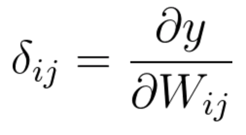
This partial derivative of the output with respect to each weight, defines the gradient and is often denoted by the Greek letter \delta.

We will find all the elements of the gradient using the chain rule.

If you are feeling confident with the chain rule and understand how to apply it, skip the next video and continue with our example. Otherwise, give Luis a few minutes of your time as he takes you through the process!